Model Metrics
This is a guide to viewing and understanding the model run metrics that are collected during Mission runtime.
After a Mission has completed, Data Scientists may want to analyze how well the Mission models learned.
After the Mission is completed Model Experiment Runs can be queried using the Fabric CLI. Data Scientists may also use the Cortex Python Library to create a workbook that offers visualizations of the queried data.
Calculated Values
When you query the model (experiment run), the following metrics calculations are displayed:
Average Reward (for policy after batch k)
"avg_reward"is the average value of reward calculated after k (some number of) batches of the Online learner have completed. Reward is measured as a continuous value between 0 and 1 that provides an indicator of how well the policy is learning. A value closer to 1 means the policy consistently picks up interventions that result in positive customer feedback; whereas, s value closer to 0 means policy is not learning effectively.Random ARM (Average Reward Metric) Baseline
"random_arm_avg_reward"is calculated by randomly assigning interventions and obtaining user feedback. This value is compared with the Average Reward of the currently running batch. If the model is learning effectively, then the Average Reward value is consistently higher than that of a randomly assigned batch."random_arm_min_reward"is the minimum value for the Random ARM Reward for the run."random_arm_max_reward"is the maximum value for the Random ARM Reward for the run.
Single ARM Baseline
"single_arm_avg_reward"is a calculated by selecting a single intervention before starting the Online Learning process and observing the rewards for that intervention after k batches. This value is compared with the Average Reward of the currently running batch. If the model is learning effectively, the Average Reward value is consistently higher than that of a Single Intervention for all runs."single_arm_min_reward"is the minimum value for the Single ARM Reward for the run."single_arm_max_reward"is the maximum value for the Single ARM Reward for the run.
Query the CLI for Calculated Values
The model metrics are are stored with the runs.
To view a list of experiments run:
cortex experiments list --project myProjectThe response looks similar to this:
┌──────────────────┬───────────────────┬──────────────────┬─────────────────────────┐
│ Name             │ Title             │ Version          │ Description             │
├──────────────────┼───────────────────┼──────────────────┼─────────────────────────┤
│ hrfsm            │ hrfsm             │ 579              │ hrfsm                   │
└──────────────────┴───────────────────┴──────────────────┴─────────────────────────┘
To obtain Model Metrics values returned as JSON run:
cortex experiments list-runs experimentName --json --limit intExample Query
NOTE: Typically you the
limitwould be much larger. The sample size is small in the example to show the complete response.cortex experiments list-runs hrfsm --json --limit 2 > metrics.jsonResponse
{
  "runs": [
    {
      "_id": "615bfa66717de7a97d894fa3",
      "runId": "craw0979",
      "_projectId": "metrics1",
      "experimentName": "hrfsm",
      "_createdAt": "2021-10-05T07:10:30.604Z",
      "_updatedAt": "2021-10-05T07:10:34.316Z",
      "endTime": 1633417834,
      "startTime": 1633417830,
      "took": 3.3553665039362386,
      "artifacts": {
        "model": "experiments/hrfsm/craw0979/artifacts/model"
      },
      "meta": {
        "algo": "SquareCB"
      },
      "metrics": {
        "avg_reward": 0.36756000000000016,
        "random_arm_avg_reward": 0.33721999999999996,
        "random_arm_min_ci": 0.04265,
        "random_arm_max_ci": 0.7594499999999998,
        "single_arm_avg_reward": 0.3812200000000002,
        "single_arm_min_ci": 0.0942,
        "single_arm_max_ci": 0.7601
      }
    },
    {
      "_id": "615bf9e070ac0e375f14f795",
      "runId": "n04g0ufh",
      "_projectId": "metrics1",
      "experimentName": "hrfsm",
      "_createdAt": "2021-10-05T07:08:16.189Z",
      "_updatedAt": "2021-10-05T07:08:19.697Z",
      "endTime": 1633417699,
      "startTime": 1633417696,
      "took": 3.122077294974588,
      "artifacts": {
        "model": "experiments/hrfsm/n04g0ufh/artifacts/model"
      },
      "meta": {
        "algo": "SquareCB"
      },
      "metrics": {
        "avg_reward": 0.36773999999999996,
        "random_arm_avg_reward": 0.3128599999999999,
        "random_arm_min_ci": 0.04285,
        "random_arm_max_ci": 0.67245,
        "single_arm_avg_reward": 0.16350999999999996,
        "single_arm_min_ci": 0.009750000000000002,
        "single_arm_max_ci": 0.46909999999999996
      }
    }
  ]
}
Use Python Notebook to display graph
You may use the cortex-python lib to create a notebook similar to the one pictured below to graph the comparison of the run metric values over time.
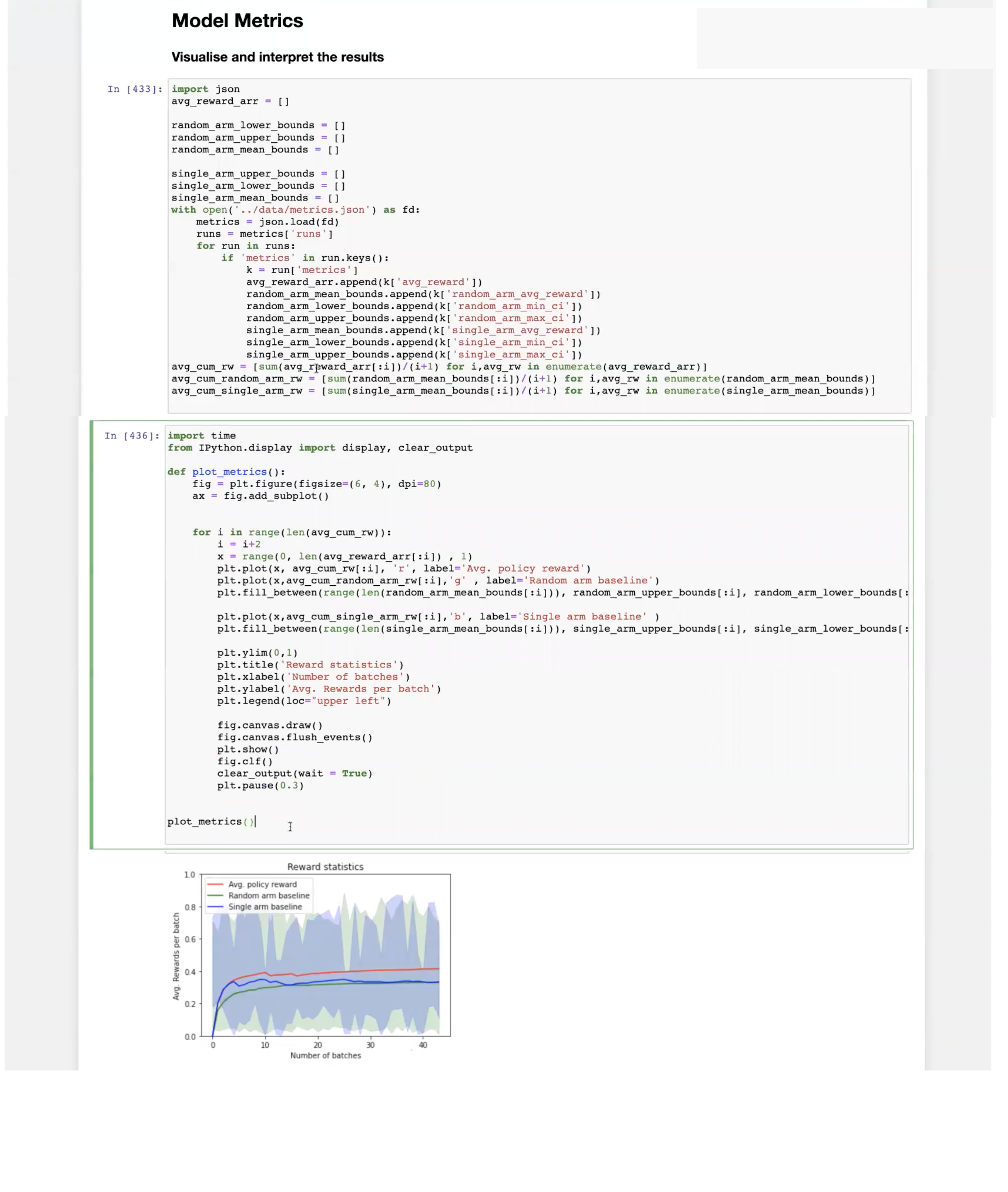
To display a graph of the Model Metric values copy the following to your Python Notebook:
In [ ]:
metrics_data_path = 'metrics.json'
In [ ]:
import json
avg_reward_arr = []

random_arm_lower_bounds = []
random_arm_upper_bounds = []
random_arm_mean_bounds = []

single_arm_upper_bounds = []
single_arm_lower_bounds = []
single_arm_mean_bounds = []
with open(metrics_data_path) as fd:
    metrics = json.load(fd)
    runs = metrics['runs']
    for run in runs:
        if 'metrics' in run.keys():
            k = run['metrics']
            avg_reward_arr.append(k['avg_reward'])
            random_arm_mean_bounds.append(k['random_arm_avg_reward'])
            rnd_arm_qnt = random_arm_mean_bounds[:]
            random_arm_lower_bounds.append(k['random_arm_min_ci'])
            random_arm_upper_bounds.append(k['random_arm_max_ci'])
            single_arm_mean_bounds.append(k['single_arm_avg_reward'])
            single_arm_lower_bounds.append(k['single_arm_min_ci'])
            single_arm_upper_bounds.append(k['single_arm_max_ci'])
avg_cum_rw = [sum(avg_reward_arr[:i])/(i+1) for i,avg_rw in enumerate(avg_reward_arr)]
avg_cum_random_arm_rw = [sum(random_arm_mean_bounds[:i])/(i+1) for i,avg_rw in enumerate(random_arm_mean_bounds)]
avg_cum_single_arm_rw = [sum(single_arm_mean_bounds[:i])/(i+1) for i,avg_rw in enumerate(single_arm_mean_bounds)]
In [10]:
import time
from IPython.display import display, clear_output
import matplotlib.pyplot as plt

def plot_metrics():
    fig = plt.figure(figsize=(18, 12), dpi=80)
    ax = fig.add_subplot()


    for i in range(len(avg_cum_rw)):
        i = i+2
        x = range(0, len(avg_reward_arr[:i]) , 1)
        plt.plot(x, avg_cum_rw[:i], 'r', label='Avg. policy reward')
        plt.plot(x,avg_cum_random_arm_rw[:i],'g' , label='Random arm baseline')
#         plt.fill_between(range(len(random_arm_mean_bounds[:i])), random_arm_upper_bounds[:i], random_arm_lower_bounds[:i], color='g', alpha=.2)

        plt.plot(x,avg_cum_single_arm_rw[:i],'b', label='Single arm baseline' )
#         plt.fill_between(range(len(single_arm_mean_bounds[:i])), single_arm_upper_bounds[:i], single_arm_lower_bounds[:i], color='b', alpha=.2)

        plt.ylim(0,1)
        plt.title('Reward statistics')
        plt.xlabel('Number of batches')
        plt.ylabel('Avg. Rewards per batch')
        plt.legend(loc="upper left")

        fig.canvas.draw()
        fig.canvas.flush_events()
        plt.show()
        fig.clf()
        clear_output(wait = True)
        plt.pause(0.5)


plot_metrics()